Matrix Mathematics
An Introduction for Computer Graphics
|
|
Prof. David Bernstein
James Madison University
|
|
| Computer Science Department |
| bernstdh@jmu.edu |

|
Getting Started
- Definition:
- An \(m \times n\) real-valued matrix
consists of \(m\) rows and \(n\)
columns of real numbers
- Some Notation:
- An \(m \times n\) matrix is usually denoted
as follows:
\(\bs{A} =
\left[ \begin{array}{c c c c}
a_{11} & a_{12} & \cdots & a_{1n} \\
a_{21} & a_{22} & \cdots & a_{2n} \\
\vdots & \vdots & \ddots & \vdots \\
a_{m1} & a_{m2} & \cdots & a_{mn}
\end{array} \right]\)
- The set of real-valued \(m \times n\)
matrices is often denoted by
\(\mathbb{R}^{m \times n}\)
- Some Terminology:
- \(a_{ij}\) is called element \(ij\)
- A matrix is said to be square if \(m=n\)
and rectangular otherwise
- Relationship to Vectors:
- A \(1 \times n\) matrix can be thought of as
a row vector and an \(m \times 1\) matrix
can be thought of as a column vector
Some History
- First Uses:
- Introduced by Sylvester in 1850 and Cayley in 1855
to simplify the notation used in the study
of sets of linear equations (i.e., the study
of linear algebra)
- The Notational Advantage:
- Consider the system of linear equations:
- \(y_{1} = a_{11} x_{1} + a_{12} x_{2} + \cdots + a_{1n} x_{n}\)
- \(y_{2} = a_{21} x_{1} + a_{22} x_{2} + \cdots + a_{2n} x_{n}\)
- \(\vdots\)
- \(y_{m} = a_{m1} x_{1} + a_{m2} x_{2} + \cdots + a_{mn} x_{n}\)
- This system can be written as:
- \(
\left[ \begin{array}{c} y_{1} \\ y_{2} \\ \vdots \\ y_{m}\end{array}\right] =
\left[ \begin{array}{c c c c}a_{11} & a_{12} & \cdots & a_{1n}\\
a_{21} & a_{22} & \cdots & a_{2n}\\
\vdots & \vdots & \ddots & \vdots\\
a_{m1} & a_{m2} & \cdots & a_{mn}\end{array}\right]
\left[ \begin{array}{c}x_{1} \\ x_{2} \\ \vdots \\ x_{n}\end{array}\right]
\)
- Or, more succinctly, as:
- \(\bs{y} = \bs{A} \bs{x}\)
- Modern Uses:
- Matrices are used in various branches of mathematics
as well as the theoretical and applied sciences
- They are central to the study of computer graphics
Transposition
- Definition:
- The transpose of the matrix \(\bs{A}\), usually
denoted by \(\bs{A}^{\mbox{T}}\), is obtained by
replacing element \(a_{ij}\) with
\(a_{ji}\)
- An Example:
- If
\(\bs{A} =
\left[ \begin{array}{c c c}
5 & 1 & 3\\
8 & 9 & 7\\
6 & 6 & 2\\
5 & 8 & 4
\end{array}\right]
\)
then
\(\bs{A}^{\mbox{T}} =
\left[ \begin{array}{c c c c}
5 & 8 & 6 & 5\\
1 & 9 & 6 & 8\\
3 & 7 & 2 & 4
\end{array}\right]
\)
- Vectors:
- The transpose of a column vector is a row vector
(and vice versa)
Multiplication by a Scalar
- Definition:
- Given \(\lambda \in \mathbb{R}\) and
\(\bs{A} \in \mathbb{R}^{m \times n}\):
-
\(\lambda \bs{A} =
\left[ \begin{array}{c c c c}
\lambda a_{11} & \lambda a_{12} & \cdots & \lambda a_{1n}\\
\lambda a_{21} & \lambda a_{22} & \cdots & \lambda a_{2n}\\
\vdots & \vdots & \ddots & \vdots\\
\lambda a_{m1} & \lambda a_{m2} & \cdots & \lambda a_{mn}\end{array}\right]\)
- An Example:
- If
\(\bs{A} =
\left[ \begin{array}{c c c}
5 & 1 & 3\\
8 & 9 & 7\\
6 & 6 & 2\\
5 & 8 & 4\end{array}\right]
\)
then
\(3 \bs{A} =
\left[ \begin{array}{r r r}
15 & 3 & 9\\
24 & 27 & 21\\
18 & 18 & 6\\
15 & 24 & 12\end{array}\right]
\)
Multiplication by a Scalar (cont.)
- Properties:
- \(\lambda (\bs{B} + \bs{C}) = \lambda \bs{B} + \lambda \bs{C}\)
- \((\lambda + \mu)\bs{C} = \lambda \bs{C} + \mu \bs{C}\)
- \((\lambda \mu) \bs{C} = \lambda (\mu \bs{C})\)
- A Warning:
Addition
- Definition:
- Given \(\bs{A} \in \mathbb{R}^{m \times n}\) and
\(\bs{B} \in \mathbb{R}^{m \times n}\):
-
\(\bs{A} + \bs{B} =
\left[ \begin{array}{c c c c}
a_{11}+b_{11} & a_{12}+b_{12} & \cdots & a_{1n}+a_{1n}\\
a_{21}+b_{21} & a_{22}+b_{22} & \cdots & a_{2n}+a_{2n}\\
\vdots & \vdots & \ddots & \vdots\\
a_{m1}+b_{m1} & a_{m2}+b_{m2} & \cdots & a_{mn}+a_{mn}\end{array}\right] \)
- An Example:
- If
\(\bs{A} =
\left[ \begin{array}{r r r}
5 & 1 & 3\\
8 & 9 & 7\\
6 & 6 & 2\\
5 & 8 & 4\end{array}\right]
\)
and
\(\bs{B} =
\left[ \begin{array}{r r r}
2 & 7 & 1\\
-1 & 4 & 6\\
3 & -6 & 7\\
1 & 1 & 1\end{array}\right]
\)
then
\(\bs{A} + \bs{B} =
\left[ \begin{array}{r r r}
7 & 8 & 4\\
7 & 13 & 13\\
9 & 0 & 9\\
6 & 9 & 5\end{array}\right]
\)
- Be Careful:
- You can only add two matrices if they are the same size
(i.e., have the same dimensionality)
Subtraction
- Definition:
- Given \(\bs{A} \in \mathbb{R}^{m \times n}\) and
\(\bs{B} \in \mathbb{R}^{m \times n}\):
-
\(\bs{A} - \bs{B} =
\left[ \begin{array}{c c c c}
a_{11}-b_{11} & a_{12}-b_{12} & \cdots & a_{1n}-a_{1n}\\
a_{21}-b_{21} & a_{22}-b_{22} & \cdots & a_{2n}-a_{2n}\\
\vdots & \vdots & \ddots & \vdots\\
a_{m1}-b_{m1} & a_{m2}-b_{m2} & \cdots & a_{mn}-a_{mn}\end{array}\right] \)
- An Example:
- If
\(\bs{A} =
\left[ \begin{array}{r r r}
5 & 1 & 3\\
8 & 9 & 7\\
6 & 6 & 2\\
5 & 8 & 4\end{array}\right]
\)
and
\(\bs{B} =
\left[ \begin{array}{r r r}
2 & 7 & 1\\
-1 & 4 & 6\\
3 & -6 & 7\\
1 & 1 & 1\end{array}\right]
\)
then
\(\bs{A} - \bs{B} =
\left[ \begin{array}{r r r}
3 & -6 & 2\\
9 & 5 & 1\\
3 & 12 & -5\\
4 & 7 & 3\end{array}\right]
\)
- Be Careful:
- You can only add two matrices if they are the same size
(i.e., have the same dimensionality)
Pre-Multiplication by a (Row) Vector
- Defintion:
- Given \(\bs{r} \in \mathbb{R}^{1 \times n}\) and
\(\bs{B} \in \mathbb{R}^{n \times p}\):
-
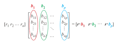
\(
\bs{r} \bs{B} = \left[ \begin{array}{c c c c}
r_{1} \cdot b_{11} + \cdots + r_{n} \cdot b_{n1} &
\cdots &
r_{1} \cdot b_{1p} + \cdots + r_{n} \cdot b_{np}
\end{array}\right]
\)
- Some Intuition:
- You can think of this as \(p\) distinct
inner products
-

- An Example:
- If
\(\bs{r} = [5 \quad 1]
\)
and
\(\bs{B} =
\left[ \begin{array}{r r r}
2 & 7 & 0\\
3 & 4 & 6
\end{array}\right]
\)
then
\(\bs{r} \bs{B} =
[5 \cdot 2 + 1 \cdot 3 \quad 5 \cdot 7 + 1 \cdot 4 \quad 5 \cdot 0 + 1 \cdot 6] =
[13 \quad 39 \quad 6]
\)
Post-Multiplication by a (Column) Vector
- Defintion:
- Given \(\bs{B} \in \mathbb{R}^{n \times p}\) and
\(\bs{c} \in \mathbb{R}^{p \times 1}\):
-
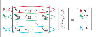
\(\bs{B} \bs{c}=
\left[ \begin{array}{c}
b_{11} \cdot c_{1}+ \cdots + b_{1p} \cdot c_{p}\\
\vdots \\
b_{n1} \cdot c_{1} + \cdots + b_{np} \cdot c_{p}
\end{array}\right]\)
- Some Intuition:
- You can think of this as \(n\) distinct
inner products
-

- An Example:
- If
\(\bs{B} =
\left[ \begin{array}{r r r}
2 & 7 & 0\\
3 & 4 & 6
\end{array}\right]
\)
and
\(\bs{c} = \left[ \begin{array}{r} 8 \\ 9 \\ 1 \end{array}\right]\)
then
\(\bs{B} \bs{c}=
\left[ \begin{array}{c}
2 \cdot 8 + 7 \cdot 9 + 0 \cdot 1\\
3 \cdot 8 + 4 \cdot 9 + 6 \cdot 1\end{array}\right] =
\left[ \begin{array}{r} 79 \\ 66\end{array}\right]
\)
Multiplication by a Vector (cont.)
- Properties:
- \(\bs{A}(\lambda \bs{v}) = \lambda A\bs{v}\)
- \(\bs{A}(\bs{u}+\bs{v}) = \bs{A}\bs{u} + \bs{A}\bs{v}\) (Distributive Law)
- A (Repeated) Warning:
Multiplication
- Definition:
- Given \(\bs{A} \in \mathbb{R}^{m \times n}\) and
\(\bs{B} \in \mathbb{R}^{n \times p}\):
-
\(\bs{C} = \bs{A} \bs{B} =
\left[ \begin{array}{c c c c}
c_{11} & c_{12} & \cdots & c_{1p}\\
c_{21} & c_{22} & \cdots & c_{2p}\\
\vdots & \vdots & \ddots & \vdots\\
c_{m1} & c_{m2} & \cdots & c_{mp}\end{array}\right]\)
- where \(c_{ij} = \sum_{k=1}^{n} a_{ik} b_{kj}\)
for all \(i=1 , ... , m\) and
\(j=1 , ... , p\)
- Some Intuition:
- You can think of this as \(m p\) distinct
inner products
-

- An Example:
- If
\(\bs{A} =
\left[ \begin{array}{r r}
5 & 1\\
8 & 9\end{array}\right]
\)
and
\(\bs{B} =
\left[ \begin{array}{r r r}
2 & 7 & 0\\
3 & 4 & 6\end{array}\right]
\)
then
\(\bs{A} \bs{B} =
\left[ \begin{array}{r r r}
5 \cdot 2 + 1 \cdot 3 & 5 \cdot 7 + 1 \cdot 4 & 5 \cdot 0 + 1 \cdot 6\\
8 \cdot 2 + 9 \cdot 3 & 8 \cdot 7 + 9 \cdot 4 & 8 \cdot 0 + 9 \cdot 6\end{array}\right] =
\left[ \begin{array}{r r r}
13 & 39 & 6\\
43 & 92 & 54\end{array}\right]
\)
- Be Careful:
- You can only add multiply two matrices if the number of columns
in the first (or "lead") matrix equals the number of rows in
the second (or "lag") matrix
Multiplication (cont.)
- An Observation:
- In general, \(\bs{A} \bs{B}\) does not equal
\(\bs{B} \bs{A}\) (i.e., matrix multiplication
is not commutative)
- An Example:
- If
\(\bs{A} =
\left[ \begin{array}{r r}
1 & 2\\
3 & 4\end{array}\right]
\)
and
\(\bs{B} =
\left[ \begin{array}{r r}
0 & -1\\
6 & 7\end{array}\right]
\)
then
\(\bs{A} \bs{B} =
\left[ \begin{array}{r r}
1 \cdot 0 + 2 \cdot 6 & 1 \cdot -1 + 2 \cdot 7\\
3 \cdot 0 + 4 \cdot 6 & 3 \cdot -1 + 4 \cdot 7\end{array}\right] =
\left[ \begin{array}{r r}
12 & 13\\
24 & 25\end{array}\right]
\)
and
\(\bs{B} \bs{A} =
\left[ \begin{array}{r r}
0 \cdot 1 - 1 \cdot 3 & 0 \cdot 2 - 1 \cdot 4\\
6 \cdot 1 + 7 \cdot 3 & 6 \cdot 2 + 7 \cdot 4\end{array}\right] =
\left[ \begin{array}{r r}
-3 & -4\\
27 & 40\end{array}\right]
\)
The Null Matrix
- Definition:
- A null matrix (or zero matrix)
is an \(m \times n\)
matrix in which each element is 0
- Notation:
- Null matrices are commonly denoted by \(\bs{0}\)
- An Example:
-
\(\bs{0} =
\left[ \begin{array}{c c c c}
0 & 0 & \cdots & 0\\
0 & 0 & \cdots & 0\\
\vdots & \vdots & \ddots & \vdots\\
0 & 0 & \cdots & 0\end{array}\right]\)
- Two Observations:
- Given any matrix \(\bs{A} \in \mathbb{R}^{m \times n}\)
and the null matrix \(\bs{0} \in \mathbb{R}^{m \times n}\)
it follows that
\(\bs{A} + \bs{0} = \bs{0} + \bs{A} = \bs{A}\)
- Given any matrix \(\bs{A} \in \mathbb{R}^{m \times n}\)
and the appropriately sized null matrices,
it follows that
\(\begin{array}{c}
\mbox{ }\\ \mbox{ }\bs{A}\mbox{ }\\ (m \times n)
\end{array}
\begin{array}{c}
\mbox{ }\\ \mbox{ }\bs{0}\mbox{ }\\ (n \times p)
\end{array}
=
\begin{array}{c}
\mbox{ }\\ \mbox{ }\bs{0}\mbox{ }\\ (m \times p)
\end{array}\)
and
\(\begin{array}{c}\mbox{ } \\ \mbox{ }\bs{0}\mbox{ } \\ (p \times m) \end{array}
\begin{array}{c}\mbox{ } \\ \mbox{ }\bs{A}\mbox{ } \\ (m \times n) \end{array} =
\begin{array}{c}\mbox{ } \\ \mbox{ }\bs{0}\mbox{ } \\ (p \times n) \end{array}\)
Division
- Of Scalars:
- Given \(a \in \mathbb{R}\) and \(b \in \mathbb{R}_{++}\)
the quotient \(a/b\) can be written as
either \(a b^{-1}\) or \(b^{-1} a\)
(where \(b^{-1}\) denotes the reciprocal or inverse)
- Of Matrices:
- Suppose, for the moment, that given
\(\bs{B} \in \mathbb{R}^{n \times n}\)
there is a notion of an inverse
\(\bs{B}^{-1} \in \mathbb{R}^{n \times n}\)
and that the inverse exists
- It may not be the case that \(\bs{A} \bs{B}^{-1}\) equals
\(\bs{B}^{-1} \bs{A}\)
- Hence, division cannot be defined without ambiguity
The Identity Matrix
- Definition:
- An identity matrix is an \(n \times n\)
matrix in which the \((i,j)\)th element is 1
when \(i = j\) and 0 otherwise
- Notation:
- Identity matrices are commonly denoted by either
\(\bs{I}\) or \(\bs{1}\)
- An Example:
-
\(\bs{I} =
\left[ \begin{array}{c c c c}
1 & 0 & \cdots & 0\\
0 & 1 & \cdots & 0\\
\vdots & \vdots & \ddots & \vdots\\
0 & 0 & \cdots & 1\end{array}\right]\)
- An Observation:
- Given any matrix \(\bs{A} \in \mathbb{R}^{n \times n}\)
and the identity matrix
\(\bs{I} \in \mathbb{R}^{n \times n}\)
it follows that \(\bs{A} \bs{I} = \bs{I} \bs{A} = \bs{A}\)
Inverse
- Definition:
- The matrix \(\bs{A}\) is said to be invertible if there
exists a matrix \(\bs{A}^{-1}\), called its
inverse, such that
\(\bs{A} \bs{A}^{-1} = \bs{A}^{-1} \bs{A} = \bs{I}\).
- Notes:
- Not all matrices are invertible
- Inverses are fairly difficult to calculate
Addition and Multiplication
- Properties:
- \(\bs{A}+\bs{B} = \bs{B}+\bs{A}\) (Commutative Law of Addition)
- \(\bs{A}+(\bs{B}+\bs{C}) = (\bs{A}+\bs{B})+\bs{C}\) (Associative Law of Addition)
- \(\bs{A}(\bs{B}\bs{C}) = (\bs{A}\bs{B})\bs{C}\) (Associative Law of Multiplication)
- \(\bs{A}(\bs{B}+\bs{C}) = \bs{A}\bs{B} + \bs{A}\bs{C}\) (Distributive Law)
- \((\bs{B}+\bs{C})\bs{A} = \bs{B}\bs{A} + \bs{C}\bs{A}\) (Distributive Law)
- \((\bs{A} + \bs{B})^{\mbox{T}} = \bs{A}^{\mbox{T}} + \bs{B}^{\mbox{T}}\)
- \((\bs{A}\bs{B})^{\mbox{T}} = \bs{B}^{\mbox{T}} \bs{A}^{\mbox{T}}\)
- A Warning (One More Time):
Addition and Multiplication (cont.)
- One Surprising Result:
- \(\bs{A} \bs{B} = \bs{0}\) does not imply \(\bs{A}=\bs{0}\)
or \(\bs{B}=\bs{0}\)
- \(\left[ \begin{array}{r r}2 & 4\\1 & 2\end{array}\right] \left[ \begin{array}{r r}-2 & 4\\1 & -2\end{array}\right] = \left[ \begin{array}{r r}0 & 0\\0 & 0\end{array}\right]
\)
- Another Surprising Result:
- \(\bs{A} \bs{B} = \bs{A} \bs{C}\) does not imply
\(\bs{B}=\bs{C}\)
- \(\left[ \begin{array}{r r}2 & 3\\6 & 9\end{array}\right] \left[ \begin{array}{r r} 1 & 1\\1 & 2\end{array}\right] =
\left[ \begin{array}{r r}2 & 3\\6 & 9\end{array}\right] \left[ \begin{array}{r r}-2 & 1\\3 & 2\end{array}\right]
\)
Determinants of 2x2 Matrices
- Definition:
- \(\left|\left[ \begin{array}{r r}a & b\\c & d\end{array}\right]\right| = a d - c b\)
- Visualization:
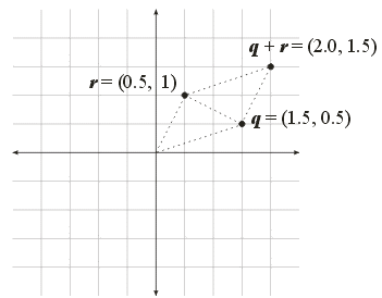
- Consider a \(2 \times 2\) matrix composed
of two column vectors \(\bs{q}\) and \(\bs{r}\):
- \(\bs{A} = \left[ \begin{array}{r r} q_{1} & r_{1}\\ q_{2} & r_{2}\end{array}\right]\)
- The determinant of \(\bs{A}\),
denoted by \(|\bs{A}|\), can be visualized as
twice the area of the triangle formed by \(\bs{q}\)
and \(\bs{r}\) (or the area of the parallelogram
formed by \(\bs{q}\), \(\bs{r}\) and
\(\bs{q}+\bs{r}\)):
-

Determinants of 2x2 Matrices (cont.)
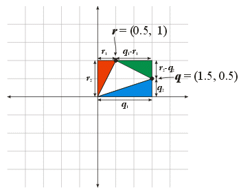
- Understanding the Visualization:
- Areas of the Colored Triangles:
- Blue: \(\frac{1}{2} q_{1} q_{2}\)
- Red: \(\frac{1}{2} r_{1} r_{2}\)
- Green: \(\frac{1}{2} (q_{1}-r_{1})(r_{2} - q_{2}) =
\frac{1}{2} (q_{1} r_{2} - q_{1} q_{2} -r_{1} r_{2} + r_{1} q_{2})
\)
- Area of the White Triangle:
- \(
\begin{align}
& q_{1} r_{2} - \frac{1}{2} q_{1} q_{2} - \frac{1}{2} r_{1} r_{2} -
\frac{1}{2} q_{1} r_{2} + \frac{1}{2} q_{1} q_{2} + \frac{1}{2} r_{1} r_{2} - \frac{1}{2} r_{1} q_{2} \\
= & \frac{1}{2} q_{1} r_{2} - \frac{1}{2} r_{1} q_{2} \\
= & \frac{1}{2} (q_{1} r_{2} - r_{1} q_{2}) = \frac{1}{2} |\bs{A}|
\end{align}
\)
Determinants of 2x2 Matrices (cont.)
- A Numerical Example:
- \(\bs{A} = \left[ \begin{array}{r r}q_{1} & r_{1}\\ q_{2} & r_{2}\end{array}\right] = \left[ \begin{array}{r r}1.5 & 0.5\\ 0.5 & 1.0\end{array}\right]\)
- \(\frac{1}{2} |\bs{A}| =
\frac{1}{2} (1.5 \cdot 1.0 - 0.5 \cdot 0.5) =
\frac{1}{2} 1.25 = 0.625\)
- A Related Example:
- \(\bs{B} = \left[ \begin{array}{r r}r_{1} & q_{1}\\ r_{2} & q_{2}\end{array}\right] = \left[ \begin{array}{r r}0.5 & 1.5\\ 1.0 & 0.5\end{array}\right]\)
- \(\frac{1}{2} |\bs{B}| =
\frac{1}{2} (0.5 \cdot 0.5 - 1.0 \cdot 1.5) =
\frac{1}{2} -1.25 = -0.625\)
Determinants of 2x2 Matrices (cont.)
- An Observation:
- The determinant can be positive or negative (or 0)
- Signed Area (The Right Hand Rule):
- If, using your right hand, you can curl your fingers from
the first column/point to the second column/point then
the area should be positive.
- This is often sometimes called the counter-clockwise rule
Determinants of Other Square Matrices
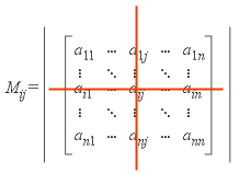
- Minors:
- The minor, \(M_{ij}\), of a square matrix
\(\bs{A}\) is the determinant of the matrix
formed by omitting row \(i\) and column \(j\)
of \(\bs{A}\)
-

- Cofactors:
- The cofactor, \(C_{ij}\), of a square matrix
\(\bs{A}\) is defined as
\((-1)^{i+j} M_{ij}\)
- Determinant:
- The determinant of an \(n \times n\) matrix
\(\bs{A}\) can be calculated using a
Laplace expansion on any row or column.
For example, expanding on row 1:
- \(|\bs{A}| = \sum_{j=i}^{n} a_{1j} C_{1j}\)
- A \(3 \times 3\) Matrix:
-
\(
|\bs{A}| = + a_{11} \left|\left[ \begin{array}{r r}a_{22} & a_{23}\\a_{32} & a_{33}\end{array}\right]\right|
- a_{12} \left|\left[ \begin{array}{r r}a_{21} & a_{23}\\a_{31} & a_{33}\end{array}\right]\right|
+ a_{13} \left|\left[ \begin{array}{r r}a_{21} & a_{22}\\a_{31} & a_{32}\end{array}\right]\right|
\)
Determinants of Other Square Matrices (cont.)
- A \(3 \times 3\) Matrix:
-
\(\bs{A} = \begin{bmatrix}
6 & 1 & 1 \\
4 & -2 & 5 \\
2 & 8 & 7 \\
\end{bmatrix}\)
- The Determinant:
-
\(
|\bs{A}| =
+ 6 \cdot \left| \begin{bmatrix}-2 & -5 \\ 8 & 7 \end{bmatrix} \right|
- 1 \cdot \left| \begin{bmatrix} 4 & 5 \\ 2 & 7 \end{bmatrix} \right|
+ 1 \cdot \left| \begin{bmatrix} 4 & -2 \\ 2 & 8 \end{bmatrix} \right|
\\ = 6 \cdot (-2 \cdot 7 - 5 \cdot 8)
- 1 \cdot (4 \cdot 7 - 5 \cdot 2)
+ 1 \cdot (4 \cdot 8 - (-2) \cdot 2) \\
= 6 \cdot (-54) - 1 \cdot (18) + 1 \cdot (36) = -306
\)
Determinants
- Properties:
- \(|\lambda \bs{A}| = \lambda^{n} |\bs{A}|\)
- \(|\bs{A} \bs{B}| = |\bs{A}| \cdot |\bs{B}|\)
- \(|\bs{A}| = |\bs{A}^{\mbox{T}}|\)
- An Interesting Example:
