• Defined:
  • In its most general usage, a convolution is a product of two functions
  • As we are using it here, a convolution is a way of calculating the color of a pixel in the destination image from that same pixel and its neighbors in the source image (the product of the source and a kernel)
• Kernels:
  • A kernel contains weights that are applied to the source pixels to obtain the destination pixels

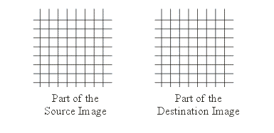
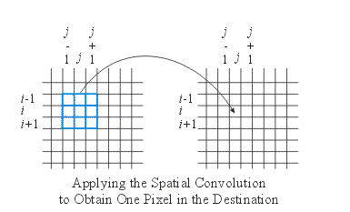
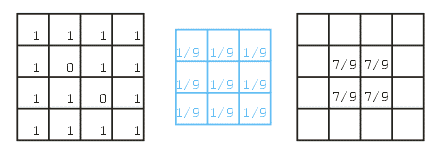
Letting \(s_{i,j}\) denote the value in source pixel \((i,j)\), \(k_{r,c}\) denote the value in element \((r, c)\) of the kernel, and \(d_{i,j}\) denote the value in destination pixel \((i, j)\), a 3x3 spatial convolution can be defined as follows:

\( d_{i,j} = \sum_{r=-1}^{1} \sum_{c=-1}^{1} s_{i+r, j+c} k_{r,c} \)

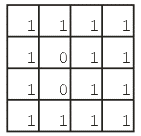
The Source

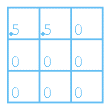
The Kernel

The Convolution

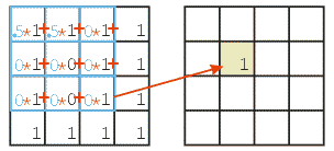
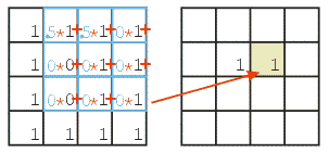
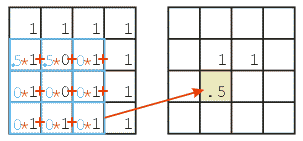
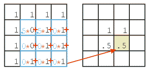
0

0

0

0

1

0

0

0

0

1/9

1/9

1/9

1/9

1/9

1/9

1/9

1/9

1/9

\( 0-1 0 -1 4-1 0-1 0 \)

• What if the value of the source pixel and its neighbors is given by \(x\)?
• What if the source pixel is brighter than its vertical and horizontal neighbors?

1. Find the edges (i.e., start with an edge detection kernel)
2. Add the edges to the original image (i.e., add an identity kernel)

1

-1

0

-1

5

-1

0

-1

1