Inferential Statistics

Inferential Statistics
An Introduction

Prof. David Bernstein
James Madison University

Computer Science Department

bernstdh@jmu.edu

Motivation

The Rumor:
- Green M&Ms are an aphrodisiac
The Impact on Someone I Know:
- He bought a lot of bags of M&Ms
What He Concluded:
- There are too few green M&Ms

Motivation (cont.)

The Data:
- There are 58 M&Ms in a bag
- There are 6 different colors
The Naive Hypothesis:
- There should be \(58/6 = 9.667\) green M&Ms in a bag
A More Sophisticated Approach:
- We should be able to use what we know about probability to calculate the expected value

Making a Probabilistic Argument

A Simpler Case:
- There are 4 M&Ms in a bag
- There are 2 different colors (red and green)
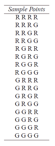
The Sample Space:

Making a Probabilistic Argument (cont.)

A Reasonable Assumption:
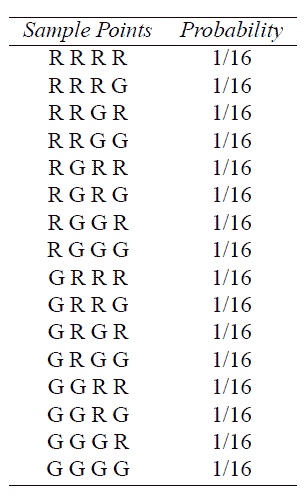
- Each outcome is equally likely
The Resulting Probabilities:

Making a Probabilistic Argument (cont.)

Creating a Random Variable:
- Remember, a random variable is a function that maps from the sample space to a set of numbers
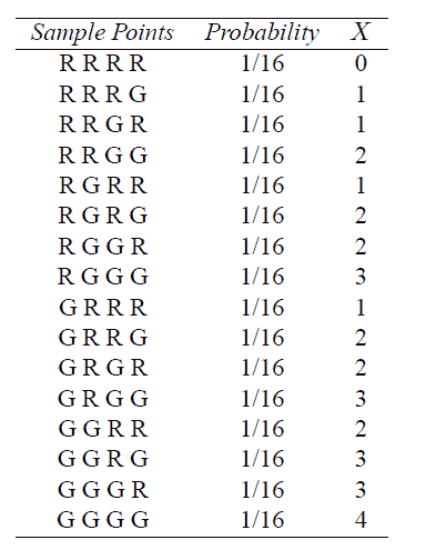
- In this case, let's let the random variable be the number of green M&Ms in a bag
The Random Variable:

Making a Probabilistic Argument (cont.)

Creating a Probability Density Function:
- Remember, a probability density function is a mapping from the possible values of the random variable to the corresponding probabilities
In This Case:
- \(f(0) = 1/16\)
- \(f(1) = 1/16 + 1/16 + 1/16 + 1/16 = 4/16\)
- \(f(2) = 1/16 + 1/16 + 1/16 + 1/16 + 1/16 + 1/16 = 6/16\)
- \(f(3) = 1/16 + 1/16 + 1/16 + 1/16 = 4/16\)
- \(f(4) = 1/16\)

Making a Probabilistic Argument (cont.)

Calculating the Expected Value:
- Remember, the expected value is the sum of the probabilities times the values of the random variable
In This Case:
- \(E(X) = f(0) \cdot 0 + f(1) \cdot 1 + f(2) \cdot 2 + f(3) \cdot 3 + f(4) \cdot 4\)
- \(= 1/16 \cdot 0 + 4/16 \cdot 1 + 6/16 \cdot 2 + + 4/16 \cdot 3 + 1/16 \cdot 4\)
- \(= 32/16 = 2\)

Interpretation

We "Expect":
- There will be 2 green M&Ms in a bag
We Realize:
- The bags are filled randomly, so any individual bag might contain fewer or more than 2
- For example, we know from the probability density function that the probability of 1 green M&M is 4/16
Implication:
- If you want to have any confidence, open more than one bag
- We can easily calculate the probabilities of different events

Back to the Real World

One Way to Proceed:
- Do the same thing for bags of 58 M&Ms in 6 colors
The Difficulty:
- The sample space contains \(6^{58}\) sample points
- (1,357,602,000,000,000,000,000,000,000,000,000,000,000,000,000)
A Better Way to Proceed:
- Inferential Statistics

Statistics

Defined:
- Numbers that are derived from a set of data
Two Important Kinds:
- Measures of central tendency
- Measures of variability

Statistics from the Population/Complete Set

Arithmetic Mean of the Population:
- \(\mu = \frac{x_1+x_2+\cdots+x_N}{N}\)
Standard Deviation of the Population:
- \(\sigma = \sqrt{ \frac{(x_1 - \mu)^2 + (x_2-\mu)^2+\cdots+(x_N-\mu)^2} {N}}\)

Statistics from the Population (cont.)

One Way to Proceed:
- Open every bag of M&Ms ever made
- See if the arithmetic mean number of greens is less than 58/6
A Better Way to Proceed:
- Work with a sample (i.e., a part of the population) and make inferences about the population
A Limitation:
- We will have to make some kind of probabilistic statement about the population

Making Probabilistic Statements about the Population

What We Need:
- A probability density function
Thus Far:
- We have assigned probabilities to sample points and used them to find the probability density function
Now:
- We want to make a probabilistic statement about a sample mean
- To do so, we need the distribution of sample means (i.e., we need the probability that the mean number of green M&Ms in any sample is, say 2, or any other number)
- So, we have to calculate this distribution

The Central Limit Theorem

Definition of the (Arithmetic) Sample Mean:
- \(\overline{x} = \frac{x_1+x_2+\cdots+x_n}{n}\)
An Observation:
- Each time we take a sample it will have a different mean
A Question:
- What is the distribution of the sample means?

The Central Limit Theorem (cont.)

The Answer:
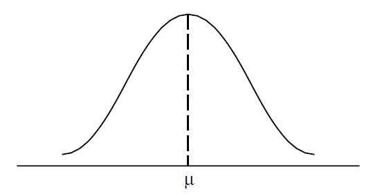
- The normal density function
- \(f(x) = \frac{1}{\sigma \sqrt{2 \pi}} e^{- \frac{(x - \mu)^2}{2 \sigma ^2}}\)
A Visualization:
Amazingly:
- The random variables do not have to be normally distributed -- as long as the random variables are independent and all have the same distribution, the distribution of sample means will tend to be normal

Back to the Simple Example

A Single Simulation:
- To simulate the purchase of 10 of our small bags of M&Ms I rolled a 16-sided die 10 times
To See the Value of the Central Limit Theorem:
- My first simulated purchase of 10 bags had a mean of 1.2 greens
- My second simulated purchase of 10 bags had a mean of 1.5 greens
- I did this 998 more times, calculating the mean each time

Back to the Simple Example (cont.)

The Frequencies

Back to the Simple Example (cont.)

The Relative Frequencies are "Bell Shaped"

The Distribution of Sample Means

The Mean of this Distribution (\(\mu_{\overline{x}}\)):
- \(\mu_{\overline{x}} = \mu\)
The Standard Deviation of this Distribution (\(\sigma_{\overline{x}}\)):
- With replacement (which we will assume):
- \(\sigma_{\overline{x}} = \frac{\sigma}{\sqrt{n}}\)
- Without replacement:
- \(\sigma_{\overline{x}} = \frac{\sigma}{\sqrt{n}} \sqrt{\frac{N-n}{n-1}} \)

Using the Distribution of Sample Means

One Particular Case:
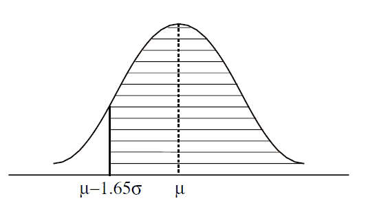
- The area under the the normal density function between \(\mu - 1.65 \sigma\) and \(\infty\) is approximately \(0.95\)
Visualizing this Case:
Using this Case:
- The probability of observing a value less than \(\mu - 1.65 \sigma\) is approximately \(0.05\) (i.e., \(1 - 0.95\))

Back to Our Example

A Hypothesis:
- The bags are "fair" (i.e., the population mean is 9.667 greens)
Suppose:
- The number of greens is normally distributed with (a mean of 9.667 and) a standard deviation of 2
Then We Know:
- The probability is less than 0.05 that any sample of bags (not any bag) has less than \(9.667 - 1.65 \cdot 2 = 6.367\) greens
Testing the Hypothesis:
- I collect a sample of bags
- The sample mean is 5 greens
- I can conclude that it is unlikely (i.e., there is a less than 0.05 probability) that the population mean is 9.667 (i.e., I can reject the hypothesis)

Back to Our Example (cont.)

An Important Question:
- How did you find the standard deviation?
A Lame Answer:
- I didn't -- I said "suppose" it is 2
An Important Open Question:
- What good is this if I have to know the standard deviation?

Estimating the Standard Deviations

Estimating the Standard Deviation of the Population:
- \(s = \sqrt{ \frac{(x_1 - \overline{x})^2 + (x_2 - \overline{x})^2 + \cdots + (x_n - \overline{x})^2 }{n - 1} } \)
Estimating the Standard Deviation of the Distribution of Sample Means:
- \(s_{\overline{x}} = \frac{s}{\sqrt{n}}\)

Using the Appropriate Distribution

An Observation:
- If we use \(s\) rather than \(\sigma\) we can't use the normal distribution
Student's \(t\) Distribution:
- Bell-shaped
- Close to normal when \(n\) is large
- "Squat" when \(n\) is small
An Implication:
- We can't use the 1.65 rule-of-thumb -- the value depends on the sample size

Using the Appropriate Distribution - Nerd Humor

\(t\) Distribution
/imgs

(Courtesy of xkcd)

Critical Values of \(t\) at the 0.95 Level

Finishing the Example

Study Design:
- I bought 20 bags of M&Ms
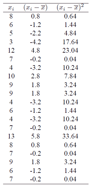
- I counted the number of green M&Ms in each and denoted the value in bag \(i\) as \(x_i\)
The Data:
- The mean was \(\overline{x} = 7.2\)

Finishing the Example (cont.)

Estimating the Standard Deviation of the Population:
- \(s = \sqrt{ \frac{(x_1 - \overline{x})^2 + (x_2 - \overline{x})^2 + \cdots + (x_n - \overline{x})^2 }{n - 1} } = \sqrt{\frac{133.20}{20-1}} = 2.65\)
Estimating the Standard Deviation of the Distribution of Sample Means:
- \(s_{\overline{x}} = \frac{s}{\sqrt{n}} = \frac{2.65}{\sqrt{20}} = 0.593\)

Finishing the Example (cont.)

Hypothesis:
- There are 9.667 green M&Ms in a bag (i.e., the population mean is 9.667)
Testing the Hypothesis at the 0.95 Level:
- \(n-1=19\) implies that the critical \(t\) values is 1.729
- This means that the probability is less than 0.05 that a sample of 20 bags will have a mean number of greens less than \(9.667 - 0.593 \cdot 1.729 = 8.642\)
- Since our actual sample mean is 7.2 we can reject the hypothesis

There's Always More to Learn