- Forward


Shading 3D Models
An Introduction


Prof. David Bernstein
James Madison University

Computer Science Department
bernstdh@jmu.edu

Print

Motivation
Back SMYC Forward
  • An Observation:
    • We commonly approximate "curved" objects with a series of "flat" polygons (e.g., triangles)
  • An Implication:
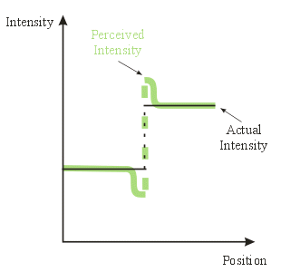
    • When we light objects they appear to be faceted
  • A Problematic Aspect of Human Vision:
    • This is made worse because, at dark-light borders, exciting and inhibiting photoreceptors do not cancel each other out
    • lateral-inhibition
Motivation (cont.)
Back SMYC Forward
  • One Resolution:
    • Use curved objects
  • Another Resolution:
    • Modify the way flat surfaces are filled (which is usually called shading)
Gouraud Shading
Back SMYC Forward
  • Approach:
    • Specify normals (that, hopefully, correspond to the normals of the curved object) at vertices
    • Determine the intensity at each vertex
    • Use a linear interpolation of the vertex intensities at each pixel
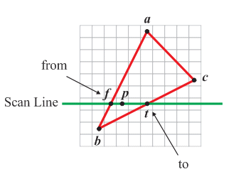
  • Visualization:
    • shading-gouraud01
  • Notation:
    • The normal at a point, \(\bs{q}\), is denoted by \(\bs{n_{q}}\)
    • The lighting intensity at a point, \(\bs{q}\), is denoted by \(I_{q}\)
Gouraud Shading (cont.)
Back SMYC Forward
  • The Intial Calculations:
    • Calculate \(I_{a}\), \(I_{b}\), and \(I_{c}\) using \(\bs{n_{a}}\), \(\bs{n_{b}}\), and \(\bs{n_{c}}\)
  • Initial Interpolations:
    • \(I_{f} = (1 - \phi) I_{a} + \phi I_{b}\)
    • \(I_{t} = (1 - \tau) I_{b} + \tau I_{c}\)
  • For Each Point on the Scan Line:
    • \(I_{p} = (1 - \pi) I_{f} + \pi I_{t}\)
    • where \(\pi = \frac{||\bs{p} - \bs{f}||} {||\bs{t} - \bs{f}||}\)
    • Note: \(\pi = 0\) when \(\bs{p} = \bs{f}\) in which case \(I_{p} = I_{f}\). Similarly, \(\pi = 1\) when \(\bs{p} = \bs{t}\) in which case \(I_{p} = I_{t}\).
Phong Shading
Back SMYC Forward
  • Approach:
    • Specify normals (that, hopefully, correspond to the normals of the curved object) at vertices
    • Use a linear interpolation of the vertex normals at each pixel
  • The Intial Interpolations:
    • \(\bs{n_{f}} = (1 - \phi) \bs{n_{a}} + \phi \bs{n_{b}}\)
    • \(\bs{n_{t}} = (1 - \tau) \bs{n_{b}} + \tau \bs{n_{c}}\)
  • For Each Point on the Scan Line:
    • \(\bs{n_{p}} = (1 - \pi) \bs{n_{f}} + \pi \bs{n_{t}}\)
    • where \(\pi = \frac{||\bs{p} - \bs{f}||} {||\bs{t} - \bs{f}||}\)
Phong Shading (cont.)
Back SMYC Forward
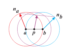
  • An Observation:
    • A convex combination of two vectors with unit length has less than unit length
  • Visualization:
    • shading-phong01
  • Implications:
    • The "interpolated normals" must be re-normalized
    • Failure to do so results in a slow algorithm for Gouraud shading [see Duff (1979)]
Shading Languages
Back SMYC Forward
  • The Idea:
    • Specify shading rules in a special-purpose language
  • Some Examples:
    • Assembly Language
    • C-like Language [e.g., OpenGL]
    • Shade Trees [e.g., Cook (1984)]
    • Declarative Languages [e.g., RenderMan]
There's Always More to Learn
Back -